Multiple Regression SPSS GSSS Dataset

Multiple Regression SPSS GSSS Dataset Project – Multiple regression is a statistical analysis technique used to examine the relationship between a dependent variable (the outcome or response variable) and two or more independent variables (predictors or explanatory variables). In other words, it allows you to predict the value of the dependent variable based on the values of the independent variables.

SPSS (Statistical Package for the Social Sciences) is a widely used software for statistical analysis in various fields, including social sciences, business, and other research domains. It provides tools to perform a wide range of statistical analyses, including multiple regression.

The GSS (General Social Survey) dataset is a well-known dataset in the social sciences, particularly in sociology. The GSS is a survey conducted in the United States that collects data on a wide range of topics, such as demographics, attitudes, and behaviors. Researchers use the GSS dataset to analyze trends and relationships in society.

Multiple Regression Background

A “Multiple Regression SPSS GSSS Dataset” refers to the application of multiple regression analysis using the GSS dataset within the SPSS software. This could involve analyzing the relationship between one or more dependent variables (e.g., income, happiness, political affiliation) and several independent variables (e.g., age, education, gender) using the GSS dataset and the statistical capabilities of SPSS.

Research question:

The effect of age, number of children, respondent’s income and weekly working hours on the overall family income.

Research hypothesis:

H_0:age, number of children, respondent’s income and weekly working hours has no effect on the family’s income.

H_1:age, number of children, respondent’s income and weekly working hours has an effect on the family’s income.

Research design:

The research design adopted in this study is referred to as causal relationship approach with the aim of analyzing the effect of age, number of children, respondent’s income and weekly working _hours on the overall family income. According to (Cooper & Schindler, 2014), the main concern in causal relationship approach is with how one variable(s) affects or is responsible for changes in another variable(s).

Dependent variable:

The dependent variable(Y) used was the family income. The income was measured in constant dollars showing how much income the whole family generates.

Independent variables:

(X₁) the first independent variable is the number of children in each family

(X₂) respondent’s income measured in constant dollars is the second variable

(X₃) weekly working hours is the last independent variable which is measured by the number of hours the respondent works in a week.

Control variables:

Control variables are the held constant in order to assess the relationship between other variables (Allison, P. D., 1990). This research has included two control variable which are the sex of the respondents and their ages. These variables are added because in a typical society the sex affects the income of the worker and the higher the age the greater the experience hence increased income. By setting the two variable as control we excluded their effect on the model.

Descriptive Statistics
	Mean	Std. Deviation	N
FAMILY INCOME IN CONSTANT DOLLARS	56199.86	48030.037	32
NUMBER OF HOURS USUALLY WORK A WEEK	39.69	12.880	32
NUMBER OF CHILDREN	2.59	1.720	32
RESPONDENT INCOME IN CONSTANT DOLLARS	31446.56	30660.828	32
AGE OF RESPONDENT	47.88	12.289	32
RESPONDENTS SEX	1.69	.471	32

Model Summary
Model	R	R Square	Adjusted R Square	Std. Error of the Estimate	Change Statistics
					R Square Change	F Change	df1	df2	Sig. F Change
1	.744^a	.554	.468	35040.004	.554	6.449	5	26	.001
a. Predictors: (Constant), RESPONDENTS SEX, AGE OF RESPONDENT, NUMBER OF HOURS USUALLY WORK A WEEK, NUMBER OF CHILDREN, RESPONDENT INCOME IN CONSTANT DOLLARS

Coefficients
Model		Unstandardized Coefficients		Standardized Coefficients	T	Sig.
Model		B	Std. Error	Beta	T	Sig.
1	(Constant)	15653.406	51982.735		.301	.766
	AGE OF RESPONDENT	1684.865	667.954	.431	2.522	.018
	NUMBER OF CHILDREN	-11618.887	4835.608	-.416	-2.403	.024
	RESPONDENT INCOME IN CONSTANT DOLLARS	.851	.330	.543	2.579	.016
	NUMBER OF HOURS USUALLY WORK A WEEK	-20.512	767.766	-.006	-.027	.979
	RESPONDENTS SEX	-21296.312	16254.030	-.209	-1.310	.202
a. Dependent Variable: FAMILY INCOME IN CONSTANT DOLLARS

Results:

A multiple regression test was carried out to test if number of children in a family, respondent’s income and number of hours worked weekly affect the overall family income. From the SPSS output the independent variable affect the dependent variable. The model summary table show that r=0.74, r²=0.554 thus, there is a positive correlation between the predictor and the response variables.

Additionally, 55.4% of the variation in the family income (M= 56199.86, SD= 48030.037, N= 32) is explained by variations in the dependent variables. From the f value F= 6.449, p=0.001, the f change tests for overall significance of the independent variable in the model and p value< 0.05 we therefore reject the null hypothesis (Anderson et al., 2000) and conclude that the independent variable are statistically significance hence they affect the family income.

The coefficient tables gives rise to the models regression equation:

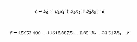
Where:

Y= family income in constant dollars

X₁= number of children in the family

X₂= respondent’s income in constant dollars

X₃= number of hours worked weekly.

e= noise

X₁(M=2.59,SD=1.720,N=32) is statistically significant at t=-2.403,p=0.024 because the p value is less than 0.05, the effect size is at -11618.887 such that an increase in children number in the family ceteris paribus leads to a decrease in family income by 11618.887dollars.

X₂(M=31446.56, SD=30660.828, N=32) is also statistically significant at t=2.579, p= 0.016 being less than 0.05 we reject the null hypothesis and conclude that the respondent’s income affects the family income. The effect size is such that an increase in the respondent’s income by one dollar ceteris paribus leads to an increase in the family income by 0.851.

X₃(M=39.69, SD=12.880,N=32) is not statistically significant, t=-0.027, p=0.979,the p-value being greater than 0.05 we accept the null hypothesis that respondent’s number of weekly working hours does not affect the family’s income.

In conclusion we establish from the statistics that, other than sex and age of the respondent the family’s income is affected by the number of children in the family and the respondent’s income holding other factors constant.

References

Allison, P. D. (1990). Change Scores as Dependent Variables in Regression Analysis. Sociological Methodology, 20, 93.

Cadotte, M. W., & Davies, T. J. (2018). Randomizations, Null Distributions, and Hypothesis Testing. Princeton University Press.

Cooper, D. R., & Schindler, P. S. (2014). Business Research Methods. New York, NY: McGraw Hill Education.

David, Anderson R., Burnham, K. P., & Thompson, W. L. (2000). Null hypothesis testing: Problems, prevalence, and an alternative. Journal of Wildlife Management, 64(4), 912-923

***Multiple Regression SPSS GSSS Datasets***

Relevant Multiple Regression SPSS Posts

Sample Dissertations

Statistics Project – Comparing Two Populations

Did you find any useful knowledge relating to multiple regression SPSS GSSS datasets in this post? What are the key facts that grabbed your attention? Let us know in the comments. Thank you.

Statistics Project – Comparing Two Populations

Statistics Project – One of the most powerful platforms in existence today is social media. The use of social media is one of the primary things that distract us as human beings, and it may have a greater influence on our thoughts and the way we go about our lives daily than we realize.

By determining the average number of hours per day that males and females spend using social media, this study aims to assess the extent to which social media impacts men and women. The number of hours people spend on social media is broken out for you in this research.

You can tell from the responses that people gave how many spend more than ten hours daily on social media. To test the hypothesis that there is no significant difference between the mean values of time spent on social media by men and women, online surveys and questions were posed to several colleagues in our college who are active on social media.

After categorizing respondents according to whether they were male or female, we next asked them a series of questions based on the average number of hours per day that they spent using various forms of social media platforms.

The data was also obtained by interviewing our colleagues in college after class. A two-sample t-test was used to examine the results of the responses. c since the p-value is less than the Alpha value.

This indicates that the null hypothesis is false and that women spend more time on social media than men do on average throughout the day. Based on this, we do not accept the null hypothesis, and there is adequate evidence to attest that this is the case.

The Question

How many hours in a day do male and female people spend on social media platforms like Facebook, Twitter, and Instagram? Is it true that women spend more time than men do on social media?

The data that was collected by sampling 40 men and 40 women says that the mean average of hours spent by males is μ= 7.125.

The significance level used is 0.05 (Alpha value)

Sampling

The sample deployed is convenience sampling because the data I obtained came from my colleagues in college. In other words, the sample comprises people who are easily accessible to the researcher. I could only collect some of the data I needed from school, so I decided to post the questionnaires online for my social media friends to fill the gaps.

I questioned a total of forty males and forty females, which gives me a sample size (n) of forty for both of the populations I was interested in. “How many hours a day would you say that you spend on social media?” was the question I posed to my friends on various social media platforms.

After I had collected some of my data, I started to inquire further by asking, “Which social networking app would you say you use the most?” This is a question I wanted to ask since I believed it would make the meaning more interesting. It would be more intriguing.

Surprisingly, the majority of the people surveyed, both male and female, claimed that Whatsapp is where they spend most of their time online. Except for the remaining subjects that I questioned my colleagues in school because they were a bit older, half of them said Instagram and Whatsapp and the other half couldn’t give an exact answer because they said that they spend the same amount of time on all of the social media that they have.

Data Table Statistics Project

Statistics Project University — ***Statistics Project – Data Table***

Statistics Two Test Sample — ***Statistics Project – Two Test Sample***

Significance Test

H0: μ1 = μ2

H1: μ1 > μ2

μ1 is the mean number of hours men spend a day on social media

μ2 is the mean number of hours women spend on social media

Hypothesis 1: The study’s hypothesis is the difference in hours taken by men and women on social media platforms.

Ho denotes the null hypothesis

The letter H1 denotes the alternative hypothesis.

Ho: There is no difference between the mean values of males and females.

H1: There is a difference between the mean values of males and females.

Hypothesis 2: The difference between the hours spent on social media by men and women

Ho: Females spend fewer hours on social media than men.

H1: Females spend three more hours on social media than men.

Hypothesis Assumptions

If the alternative hypothesis, H1, is correct, we can deduce that women spend more of their waking hours on social media than males. Assuming that the alternative hypothesis is correct, we may deduce from the data that the mean and average values are extremely different.

P – Value

A statistical test will produce a p-value, a probability that informs you how likely it is that you found a particular data set, given that the null hypothesis is correct. This probability is determined by the test results (Pagano et al., 2022).

The P value for the study is 0.00837, which is less than the alpha value (0.05); therefore, we reject the null hypothesis. We conclude that the alternative hypothesis is correct.

Significance Test Conclusion

Because the P-value is lower than the significance level, we have concluded that the null hypothesis should be rejected. We conclude that there is a significant level even though we reject the hypothesis known as the null hypothesis, which states that there is no difference between the means.

Sampling Method Strengths

The sampling method used in this case was an effective one. By combining convenience sampling and online surveys, I could reach a large sample size of 80 people, both male and female. This allowed for the results to be more reliable and valid.

Moreover, by asking specific questions regarding the use of social media, I was able to obtain more detailed data and draw more meaningful conclusions. Overall, this sampling method provided the necessary data to analyze and draw conclusions.

Weaknesses

The sampling method used in this case also had some weaknesses. The main weaknesses of this method are the lack of randomization and the lack of representative sampling. It could not access a representative sample of the population by relying mainly on convenience sampling and online surveys.

Furthermore, the lack of randomization meant that it could not be certain that the sample accurately represented the whole population. Additionally, it could not obtain data from certain groups, such as the elderly, which could have provided additional insight into the use of social media. Therefore, the sample used in this case needed to be more representative.

What Could Be Done Differently?

If I were to do the study again, I could use a more comprehensive sampling method. Instead of relying mainly on convenience sampling and online surveys, I could use a combination of different sampling methods, such as stratified sampling and random sampling.

This would allow us to obtain a more representative sample of the population and ensure that the sample accurately represents the whole population. Additionally, I could use a larger sample size to increase the reliability and validity of the results. Furthermore, I could use a different set of questions or survey methods to gain a deeper understanding of the use of social media.

Overall, a more comprehensive sampling method would allow me to obtain more accurate and detailed data, ultimately leading to more meaningful conclusions.

Extraneous Variables, Which Became an Issue

One extraneous variable I had yet to anticipate was the age of the subjects. As I relied mainly on convenience sampling and online surveys, I needed help accessing a representative sample of the whole population. This is because certain age groups, such as the elderly, were not included in the sample due to the lack of access.

Additionally, certain age groups may use social media differently from other groups, which could lead to inaccurate results. Furthermore, the lack of randomization meant that certain age groups may have been over- or under-represented in the sample, which could have impacted the results.

How To Resolve

If I were to do the project over, I would use a combination of different sampling methods to obtain a more representative sample of the population. Specifically, I would use a combination of stratified and random sampling to ensure that the sample accurately represents the whole population.

Additionally, I would use a larger sample size to increase the reliability and validity of the results. Furthermore, I would also use a different set of questions or survey methods to obtain a deeper understanding of the use of social media. Overall, using a more comprehensive sampling method would obtain more accurate and detailed data, ultimately leading to more meaningful conclusions.

Extrapolation

I am comfortable extrapolating my results to the population of young adults aged 18-25 years old. This is because this was the age group that was mostly represented in my sample. Additionally, this age group is most likely to be the main social media users, as they are more likely to be tech-savvy and use social media more frequently than other age groups.

Moreover, this age group is also the most likely to be impacted by the use of social media, as they are in the process of establishing their identities and are more likely to be influenced by the content they see online. Therefore, I am comfortable extrapolating my results to this population.

Conclusion

This study found that males and females use social media differently. Women spend more time on social media than males, the research found. This means women are more influenced by social media and internet information. The study emphasized employing a broad sampling approach to get accurate results.

By combining sampling methods, a more representative population sample can be obtained, leading to more valid results. This study sheds light on social media use and its impact on individuals.

This study reveals gender variations in social media use. It shows the need for a comprehensive sampling approach and that males and females use social media differently. This study’s conclusions can be utilized better to understand social media’s effects on individuals and target messages and content to different groups.

References

Pagano, M., Gauvreau, K., & Mattie, H. (2022). Principles of bio-statistics. CRC Press.

Relevant Statistics Project Posts

Unemployment, Inflation and Production

Dissertation Samples

If you enjoyed reading this statistics project post, I would be very grateful if you could help spread this knowledge by emailing this post to a friend, or sharing it on Twitter or Facebook. Thank you.

Trend Forecasting Steps For Analysis

Trend Forecasting Steps

Fashion forecasting is generally a career that involves focusing on upcoming trends in the fashion industry. Fashion and trend forecasting is the future determination of mood, behavior and purchasing habits of consumer at a given time of season. It does not only involve determination of markets, consumers in terms of age, their locations and income but also inquire deeply to get to know what they purchase depending on their culture, beliefs, moods as well as geographical location. Fashion and trend forecasting is more reliant on fashion cycle and plays a significant role in introductory stage of consistent fashion cycles.

Fashion and trend forecasting involves a series of activities in each of the area it is dealing with. For example it looks at the; season, target market, consumer, colors, fabrics, silhouette, texture and usage. Therefore, comprehending fashion and trend forecast is not only crucial in determining the success of the ultimate object of the designer but also enhances the continuous repetition of sales in future seasons as well as promoting the fashion cycles.

Unlike in the past when trend forecasting was done manually, current trend forecasting is done using technological forecasting methods although they have been criticized for reducing creativity by most designers. Most trend forecasting are determined by the forecasting method applied by the ultimate user and it is therefore crucial to determine the most appropriate method of trend forecasting in any individuals business model. Generally, any trend forecasting methods involve the following steps (Hines, 2007);

The first step is Problem definition. Although this is the hardest section of forecasting, it is the most important. This step requires keen analysis of how the forecasts will be used, who needs the forecasts as well as how the forecasting technique suits within the firm needs the forecasts. A forecaster should therefore use enough time to every individual who will take part in data collection, keeping the data as well as applying the forecast for future planning. Then gathering of information follows whereby in most cases, statistical or quantitative data and qualitative data are the ones required. Therefore, the collectors of the data should be expertise who can be able to receive the qualitative information from the respondents who are usually the customers if there is no adequate quantitative information (Wong, 2010).

The third step is preliminary analysis, also called exploratory analysis. In this step, the forecaster should consider whether or not there are consistent pattern that lead to significant trend, whether or not there is evidence of business cycles, the presence of outliers in the information that need explanation as well as the extent of relationship between variables present for analysis.

The fourth step is choosing and fitting models. The best method of trend forecasting should depend on the historical data present, the application of the forecasts as well as the extent relationship between the forecasts available and explanatory variables. Some of the methods that can be arrived at includes; exponential smoothing model, ARIMA model, vector autogression, neural networks among others (Wong, 2010).

The last step involves the use and evaluation of the forecasting model. The success of the model can only be determined after the data for the forecast time has been present after which various methods are applied to assess the success of the model.

Research Methodologies

As earlier stated, the main data required in trend forecasting is qualitative, quantitative and mostly commonly, a combination of the two.

The quantitative research methodology start right from the bottom, where agencies and even the manufacturers either inquires directly from the customers on their purchasing preferences or the organization may record the consumers buying habit in a duration of a given time. The consumer’s response is recorded and used to determine preference for some specific garments, accessories or any other product on research, colors, and sizes among other factors of a product. Surveys through mail, customer response or phones are carried through publication as well as contracting market research organizations for manufacturers and as well as retailers.

The survey questions usually relate to life style, income, shopping habits as well as fashion preference. The customers who participate in these surveys are selected by the research company although they should suit with manufacturers or retailers requirements. Informal discussion with consumer enable researchers get information through asking questions to customers about what they would prefer to purchase, the types they prefer to purchase which is currently present as well as the change in products they require and are not available or they cannot reach. Most researchers use small scale retailers because of their contact and conversation with the customers.

The quantitative methodology entails the use of statistical data or information to determine the trend in customer demands and hence forecast on producing what the consumers purchase the most. Statistical data for fashion sector is easily obtainable without necessarily going to the field because it is available in manufacturers or retailers sales records (Hines, 2007).

From such records, the manufacturers can determine which garments, color of the product, size as well as the fashion preference of the consumer. After that, the manufacturer should be able to determine which fashion product should be produced more depending on sales experienced at each season of the year. It is valuable noting that a well-balanced combination of the qualitative and quantitative research methodologies is bound to boost the success of the model selected for trend forecasting.

Conclusion

This paper has attempted to show that the fashion industry has one main purpose; to offer desirable as well as appealing product to not only satisfy the customer needs, demands and aspire to have them but to also keep the product selling in the subsequent business cycles with a similar season. Every successful trend forecast must commence with the consumer through determination of the consumer’s needs to the market as well as the ability to make the consumer adjust the marketplace to his preferences and lifestyles. The paper has also expounded on the two critical methodologies used in forecast research i.e. the qualitative and quantitative methodologies. It has also emphasized on the need to combine the two methods in order to attain the best results of the model of forecast selected.

References

Hines, T., & Bruce, M. (Eds.). (2007). Fashion marketing: contemporary issues. Routledge.

Wong, W. K., & Guo, Z. X. (2010). A hybrid intelligent model for medium-term sales forecasting in fashion retail supply chains using extreme learning machine and harmony search algorithm. International Journal of Production Economics, 128(2), 614-624.

Relevant Blog Posts

Marketing Fashion Dissertation

Fashion Industry Economy

Marketing Dissertation Titles

Thanks for taking the time out to read this blog post and I hope you found it useful. I would be grateful if you could share this blog post via Twitter, Facebook, or Google+ I would like to generate as much social media buzz around this post.